The download link has been removed so that GitHub stops complaining.
The program is executed as a2 <file> [<threshold>]. If no threshold is specified, a default of edge-based adjacency will be used. Note that calculating adjacency with thresholds will incur a significant startup cost.
The mesh viewer implemented for this is very simplistic, using only the fixed function pipeline and no performance optimizations to enable easier manipulation of the mesh data. Thus, for detailed meshes, expect there to be some visual lag until the mesh has been reduced.
The view may be rotated with a left click and drag. The trackball rotation calculation was pulled from a previous CSE 167 assignment.
The view may be panned with a right click and drag.
The view may be zoomed using the mouse wheel.
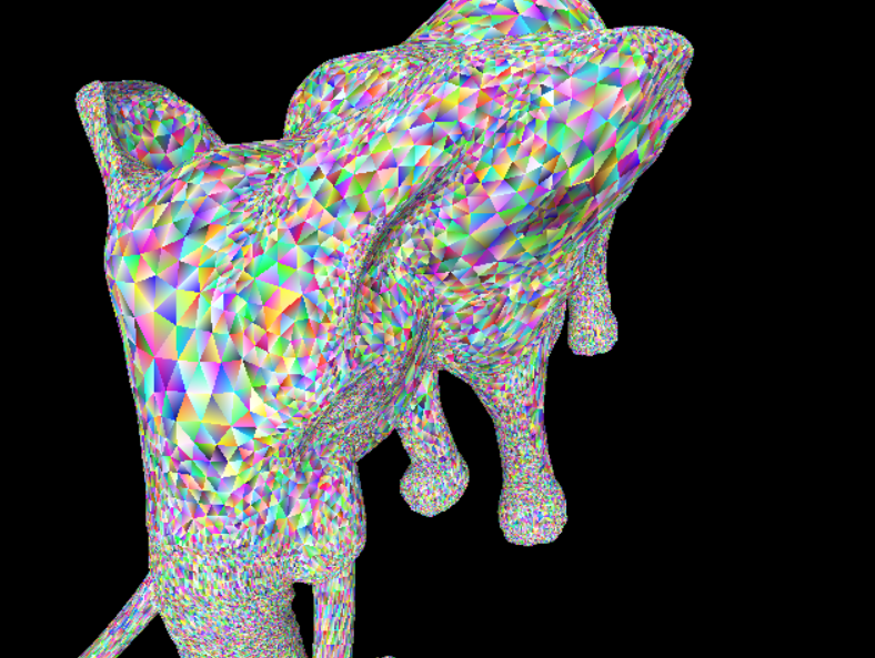
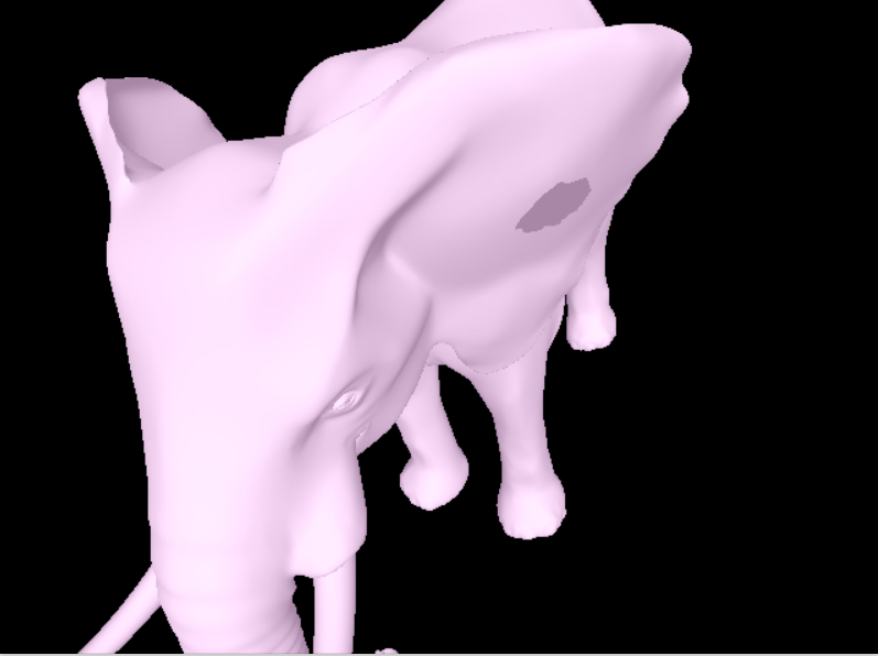
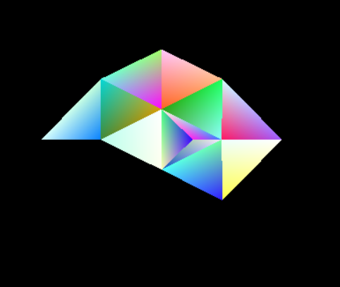
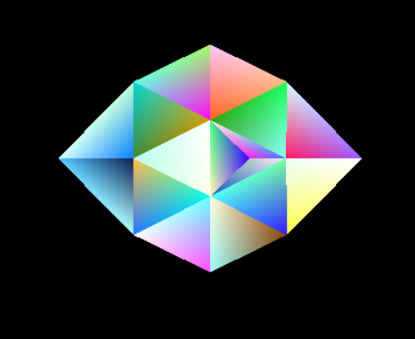
In order to enable debug colors, hit the 'd' key. This will enable a sort of gemstone appearance, in which each vertex of each face has a different color value (however, this will not be the same color for the same vertex in multiple faces). The default view is shaded based on the normals calculated based on face orientation. Note that there is an unexpected which will cause the color of the model to no longer be grey after toggling debug view.
The data structure used was an indexed vertex list coupled with a face list. Each vertex in the vertex list maintains a list of the faces of which the vertex is a part, and this allows the vertices to keep track of their neighbors.
This structure was selected due to the simplicity of implementation. This is the most convenient structure to send to OpenGL, and so using this structure minimizes the amount of transformation required in order to display the data. It is also reasonably efficient for edge collapses; these are implemented by replacing the first of the two vertices with the new vertex, thus maintaining that index, and then replacing the references to the second vertex with the index for the first, thus preventing the need to correct indices for all subsequent vertices and simplifying the progressive mesh process. Thus, this remains a O(f) process, where f is the number of faces involved with the second vertex. The faces are combined by adding them to a red-black tree in order to prevent duplicates, which is then converted back to an array when all faces in the merge have been processed. This brings the data structure merge to an O(f log(f)) process.
Creating the data structure is very straightforward. As each vertex line is read, the data is parsed and the vertex is placed into the vertex list. The faces are then read in the same manner, with each vertex given a reference to any faces which contain it. As faces are being read, data is aggregated for calculating the normals. After all the faces are read, the data is then normalized and the normals are assigned to the appropriate vertices. After this, the error matrices are calculated for each vertex, the model is scaled and centered, and the connecting pairs are determined.
Mesh decimation is mostly described above. One thing to note is that degenerate faces are not discarded from the data structure, but are instead marked as invalid; when drawing the model, the program checks each face for validity before attempting to draw it. The idea behind this was that this would make the progressive mesh more straighforward, as the face does not need to be reconstructed, but instead just marked as valid again.
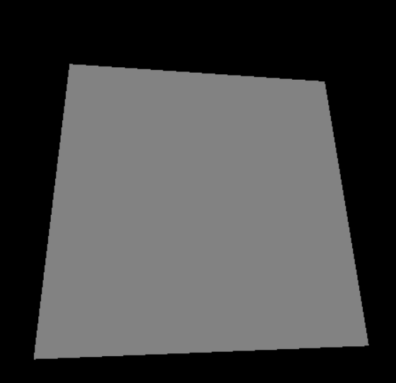
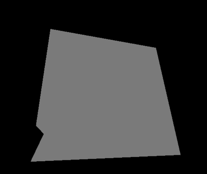
Simple edge collapse may be done manually by hitting the 'e' key, typing the index of the first vertex followed by the enter key, and then typing the index of the second vertex followed by the enter key. This will combine the vertices to the midpoint; in order combine to first vertex as displayed below, the code was temporarily modified. After the 'e' key is hit, a prompt will be displayed to the command prompt (if available); note that the graphic window must be selected in order to have your input understood by the program.
A heap was implemented in order to perform the simplification. Each vertex keeps a record of the pairs of which it is a part, and each pair keeps a record of where it lies in the heap. This allows pairs to rapidly be accessed, modified, and re-sorted.
Quadric simplification is controlled through the 'x' and 'c' keys. The 'x' key will remove a single vertex and report the number of milliseconds required to do so. The 'c' key will reduce the mesh to 10% of its original vertices and report the time required to do so in seconds.
Optimal vertices are calculated. However, this is not a perfect implementation, as can be seen below.
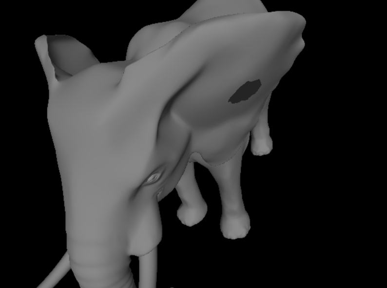
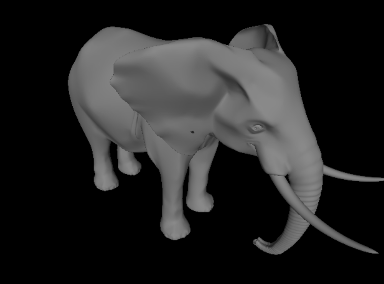
Pictured below is the elephant model before and after decimation (reduced to 10% of its original vertices). This process took about 37 seconds, tracked by the program.

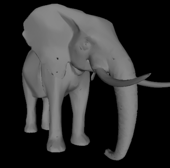
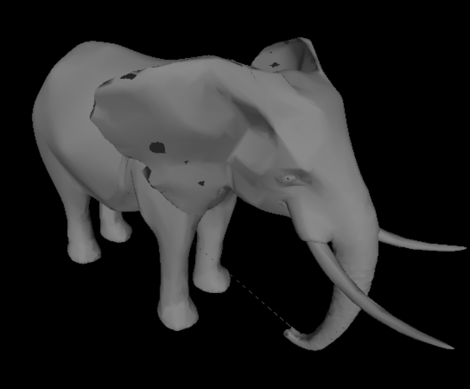 The image
on the left is the elephant prior to decimation. The image on the right is the
elephant after decimation. Notice the shading artifacts created during the decimation
process as well as the chunk taken out of the elephant's ear.
The image
on the left is the elephant prior to decimation. The image on the right is the
elephant after decimation. Notice the shading artifacts created during the decimation
process as well as the chunk taken out of the elephant's ear.
Difficulties with this portion arose mostly due to simple errors which had profound effects - adding instead of multiplying in the matrix * vertex implementation and neglecting to dereference pair pointers were two small errors which took quite a bit of time to locate.
This was implemented through an internal data structure rather than through a separate file. This removes the need to reparse the data and allows for a more fluid experience. For each split, an internal record keeps a snapshot of the data before and after the split. This requires a solid chunk of memory, although means that splist do not need to be recomputed after the mesh has been reconstructed.
In order to progress through the progressive mesh, the 'x' and 'z' keys may be used. After at least one edge collapse has been enacted, the 'z' key may be used to regenerate the mesh. If the 'x' key is hit after the 'z' key, then an undone split will be reapplied, but not recalculated. Information will be sent to the terminal about where the user stands in the calculated splits.
Below is a video demonstrating the progressive mesh. If it does not load, it may be found on YouTube here.